One of the challenges of working on a live banking application that handles millions of transactions a day is that the larger the amount of data, the harder it is to query it. Here’s how my development team extracted and transformed the data so we could query the transactions we needed.

Because we’re in the financial sector, which the government regulates, delegated government auditors need unrestricted read access to our transaction data. They need integrity and consistency of the data, so they can read and query it when required.
We used Extract, Transform and Load (ETL), a big data technique, to store and transform the data so the auditors could easily query and analyse it. ETL is the process that transforms raw data into structured, ready-to-query data on a schedule or on-demand basis.
Why we had lots of messy data
Before understanding how to process data, let’s glance at the raw data we process. We call it raw data because it’s unprocessed: Most of the time, rows in a table store each transaction.
| id | user_id | to_user_id | amount | currency | date |
| 1 | 1 | 2 | 10 | EUR | 2022-10-15 22:00:00 |
| 2 | 1 | 3 | 10 | USD | 2022-10-15 23:00:00 |
| 3 | 3 | 2 | 1 | RON | 2022-10-15 23:30:00 |
In the example above, we see the transactions: payments that took place, from one user to another, with the amounts and dates. Usually, we also store any promotions, ticket IDs (for pre-pay) or IDs of third-party vendors that are integrated with our payments. This way, with each payment, we store a unique transaction and make sure we can reconstruct the flow of money.
Data becomes messier and messier, leading to two problems:
- We can’t query this table because it changes a lot; literally, millions of new transactions are added throughout the day
- It’s a lot of data to process, even for large servers with a lot of resources
Before we could tackle our problems, we needed to make some decisions about data storage.
Why we chose a data lake for storage
The transactions table has a high number of INSERT operations. One INSERT operation is the same as adding a new transaction. With each INSERT operation, we tell the database, “please add this data to a new row in THAT specific table”. When relational databases comply with this INSERT operation, they have to write that data on disk, so we don’t lose valuable, actual transactions. Querying or reading large amounts of data means we then have to retrieve that data from the disk. Because that disk was writing a new row each millisecond, it slowed down our live database when we tried to query or read data. This led to a general slowdown of our app—something we needed to avoid as we were working on a live app.
Most databases that read or write on disk have in-memory caching: If you run the same query for a second time, you’ll retrieve the data faster because it was kept in memory. But this applies only if the data didn’t change in the meantime. In our case of adding new transactions every few milliseconds, this didn’t work.
We first needed to offload the transactions out of the system to a data lake to fix this problem.
Data lakes are places where you can store your data for long periods. You can’t query data lakes without prior tools and techniques because the data is usually unstructured files stored on a disk somewhere in the cloud. Data lakes are normally found in an object-storage service like AWS S3 or Google Cloud Storage.
We decided to store the data in a data lake for two reasons:
- To partition it on-demand, using ETL jobs that will read the stored raw data from the bucket and structure it better so that we can load and query only the data we need.
- Laws require us to have raw transactions for several years, usually ten or more years, before we can archive or discard them. Object storages like AWS S3 or Google Cloud Storage services are the best choice because their long-term reliability is so high.
The next step to solving our problem was to have a batch job that partitions the data, leading to setting up a system and running queries on the partitioned data. This would be much faster and wouldn’t interfere with our live database, and we could save queries, so we didn’t have to run them multiple times.
Partitioning data helps us focus on the data we need
With big data involving hundreds of terabytes, you can often end up with a lot of useless information if you’re querying unpartitioned data. For example, if I want to see a specific customer’s transactions for a day, querying unpartitioned data would mean loading and going through all transactions for that day. 99.9% of that data will be useless since we have millions of customers but we might only need three specific records.
The partitioning process is useful because it allows us to, as the name implies, split the data into parts that we can still load later. In our case, though, we loaded just the data we needed. The data required was for a specific period based on dates the government officials auditing us wanted.

ETL: Extract, Transform, Load
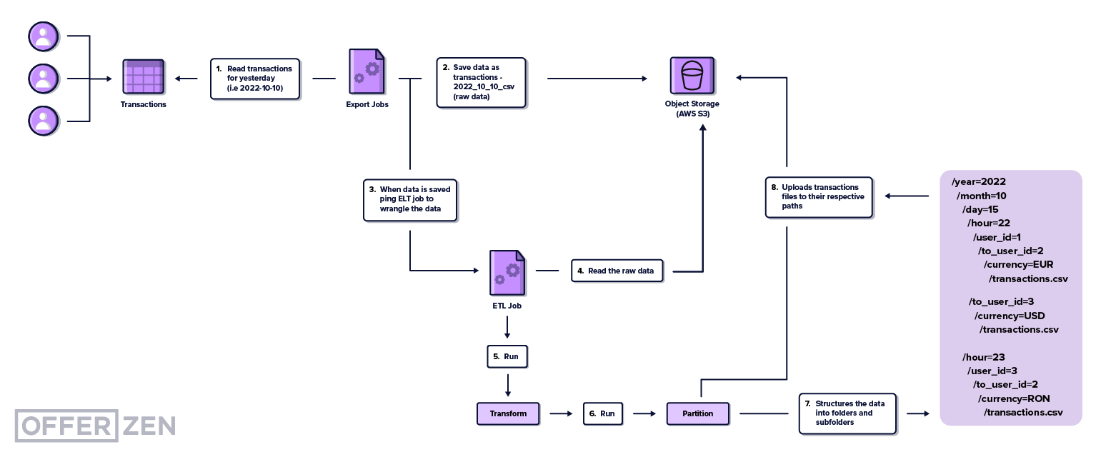
Once we partitioned the data and added it to the data lake, we were ready to follow the ETL technique: extract, transform and load it. The ETL process enabled us to take the raw data and make it easy to query.
Extracting the data
In our case, extraction was the step in which we pulled the data from the bucket. The bucket is where all the raw and partitioned data’s stored—either using AWS S3 or Google Cloud Storage.
Extracting the data is a fundamental part of the ETL process because we have to transform the CSV file with millions of records to change its format to a version that can be queried faster and easier. We process our data here only once and decouple it, so it doesn’t interfere with the live database and ultimately slow down users.
Transforming the data to query it
To understand the transform part, let’s talk a bit about how the raw data gets saved to the data lake:
id,user_id,to_user_id,amount,currency,date
1,1,2,10,EUR,2022-10-15 22:00:00
2,1,3,10,USD,2022-10-15 22:30:00
3,3,2,1,RON,2022-10-15 23:00:00
This is a brief example, just three records, which most computers would take milliseconds to read and partition. When we talk about millions of records, though, things slow down significantly. To combat this, we run Apache Spark, special software that manages transforming tasks. We send the path to the raw CSV and tell it to ignore certain fields or create a new partition path based on particular fields:
import pyspark
from pyspark.sql import SparkSession

spark = SparkSession.builder \
            .appName('OurCoolPartitioner.com') \
            .master("local[5]") \ # 5 parallel chunks
            .getOrCreate()
Apache Spark can distribute this task, meaning that if we have five million records and five servers, five million records are split among five servers, so each server is allocated one million files. Each server can process the records in parallel, making the final partitioned data available faster.
The transformation process may take a lot of time, depending on how much data you have and how often you do it. For us, doing it daily was enough because that’s what was needed to build up the reports for government authorities. The time to process the data differs, depending on how much data there is and how many Apache Spark servers you’ve got that can process the parallelisation. Therefore, the speed increases linearly with the number of servers you add.
Loading the data
Once we have properly partitioned data into folders and subfolders, we move to the load step. Here we tell the servers, “once you’re done, put the partitioned data back into the data lake in a separate location so that we can differentiate between what is raw and what is partitioned”. This way, we can query the partitioned data efficiently using dedicated services and software like Google Big Query.
Big Query is one of the native big data solutions in Google Cloud. We chose it solely because it’s already integrated with our storage and is proven to work well without any additional maintainence. We just create a Big Query table, configure the location that should look after partitioned data, and can query it through their HTTP API or from the Google Cloud Console in the browser.
The load step enables us to read up to 99% less data and query it in a few seconds, which is major progress compared to how we initially did this with raw data.
Quering our partitioned data
Let’s take a look at our example once more:
id,user_id,to_user_id,amount,currency,date
1,1,2,10,EUR,2022-10-15 22:00:00
2,1,3,10,USD,2022-10-15 22:30:00
3,3,2,1,RON,2022-10-15 23:00:00
When we ran our transform and load steps, we told the servers: “when you read these files, make sure to partition by year, month, day, hour, minute, user_id, to_user_id and currency”. This enabled us to query only the data we needed for auditing purposes.
Here’s what the query looked like:
import pyspark
from pyspark.sql import SparkSession

spark = SparkSession.builder
            .appName('OurCoolPartitioner.com') \
            .master("local[5]") \ # 5 parallel chunks
            .getOrCreate()

data = spark.read.option("header",True) \
            .partitionBy(“year”, “month”, …the rest of the fields) \ # 2. partition by this
            .mode(“overwrite”) \
            .csv("gcs://path-to-bucket/raw_data") # 1. read this file
It’s a pretty long list, but the servers understood what they should do. After they partitioned the data locally, on their own disks, they re-uploaded the files in folders like this:
transactions/year=2022/month=10/day=15/hour=22/minute=0/user_id=1/to_user_id=2/currency=EUR/data.csv
transactions/year=2022/month=10/day=15/hour=22/minute=30/user_id=1/to_user_id=3/currency=USD/data.csv
transactions/year=2022/month=10/day=15/hour=23/minute=30/user_id=3/to_user_id=2/currency=EUR/data.csv
This is a special format, called Hive Partitioning, that basically links a filesystem-like path, like Windows or Linux, with key-value sets. In the folder and subsequent folders that are under year=2022, you will find only data that has been processed in that respective year. In the same way, under user_id=1, we will find only data from that respective user.
If we need the data for the user with ID=1, we will run something like this in Google Big Query:
SELECT * FROM transactions WHERE user_id = ‘1’;
Because we partitioned our data, it will read only files from the following path:
transactions/*/*/*/*/user_id=1/*/*/*.csv
This excludes a lot of unnecessary data, because it knows directly where the files are that we want to load—which in turn make our query fast and resource-efficient.
With partitioning, we also managed to keep the costs low as we load only the data we need. There’s no unnecessary data in the table and the runtime isn’t as costly in terms of Cloud pricing.
As a result, our team was happy: We managed to minimise the impact on the live services while having the safety needed by the law, and making our data easy and quick to query.
Resources
Related Reading
Alex is a minimalist Laravel developer, full-stacking with AWS and Vue.js and sometimes deploying to Kubernetes. 🚢 He’s the mastermind behind @soketirealtime, a college dropout and open sourcerer 🧙♂️ dedicating his life to share knowledge and useful code. He also helps businesses migrate to the cloud and implement better solutions with the Laravel ecosystem.